GATEの使い方 5 ~結果の出力と表示~

How to use GATE 5

admin_bear

今回は結果の出力方法と表示についてです。
This article focus on output and display of the results.

シミュレーションは情報を取り出さなければ意味がありません。GATEではいくつかの形で情報を取得し、出力することができます。
Simulation has no meaning without extracting information. GATE can acquire and output information in several ways.

これを読めば計算結果の出力について知ることできます！
You can know how to get and display the results of simulation if you read this article.

GATEの使い方 5
How to use the GATE

出力形式の指定
　　　Specify the output format

GATEでシミュレーションを行う場合、目的に最も近いサンプルコードをもとにスタートします。
When simulating with GATE, you need to select the sample code considering your own purpose, and edit it.

それぞれのサンプルコードはシステムの構成が決められています。
システムの構成はこちら。
The system configuration is determined for each sample code.
See here for the system configuration.

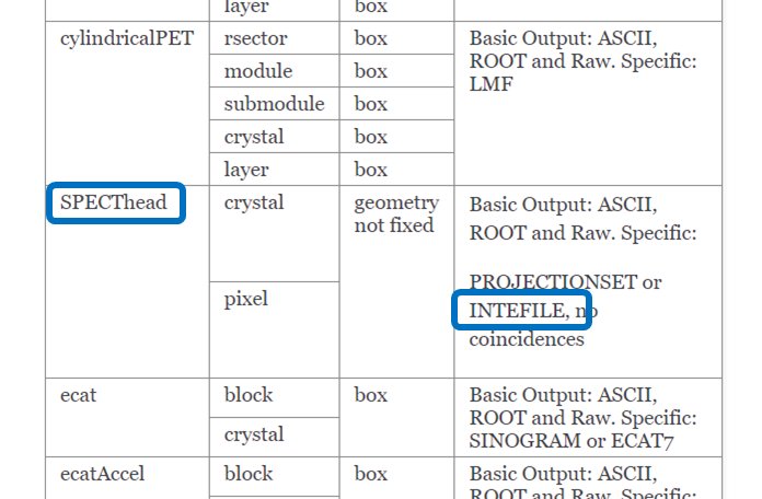
例えば
「CylindricalPET」は5つのコンポーネントから構成される
The sample (“CylindricalPET”) is consisted by five components.

1. rsector <box> (depth=1)
2. module <box> (depth=2)
3. submodule <box> (depth=3)
4. crystal <box> (depth=4)
5. layer[i] i=0~3 <box> (depth=5)
Type of the output：ASCII、ROOT、Raw、LMF

「ecat」は2つのコンポーネントから構成される
※EcatシステムはCylindricalPETの簡易版
The sample (“ecat”) is consisted by two components.
P.S. Ecat is a simplified version of CylindricalPET.

1. block <box> (depth=1)
2. crystal <box> (depth=2)
Type of the output : ASCII、ROOT、Raw、sinogram、ECAT7

「SPECThead」は2つのコンポーネントから構成される
The sample (“SPECThead”) is consisted by two components.

1. crystal <free> (depth=1)
2. pixel <free> (depth=2)
Type of the output：ASCII、ROOT、Raw、PROJECTIONSET、INTEFILE

配置したコンポーネント（Volume）はシステムにattachする必要があり、下記のようにします。
You need to attach placed components to the system, as bellow.

/gate/systems/cylindricalPET/rsector/attach              detector_blocks
/gate/systems/cylindricalPET/module/attach               block
/gate/systems/cylindricalPET/crystal/attach              crystal

その上でVolumeをSensitive detector (SD)に登録します
Moreover, you have to register volume to sensitive detector (SD).

/gate/crystal/attachCrystalSD
/gate/phantom/attachPhantomSD

最後に保存するデータを指定します。
データ形式も指定します。（ROOTやASCIIなど）
その方法をこれから説明していきます
Finally, you specify the kind of save data and type of output (ROOT or ASCII etc…).
I show how you specify the methods bellow.

ASCII形式（推奨しない）
　　(not recommended)

/gate/output/ascii/enable
/gate/output/ascii/setFileName  OUTPUTNAME
/gate/output/ascii/setOutFileSinglesAdderFlag 0
/gate/output/ascii/setOutFileSinglesBlurringFlag 0
/gate/output/ascii/setOutFileSinglesThresholderFlag 0
/gate/output/ascii/setOutFileSinglesUpholderFlag 0

CylinderPETのコードの中に上のような記述をすると、以下のものが出力されます。
You can get these result when you write above command in your macro.
・OUTPUTNAMERun.dat
・OUTPUTNAMEHits.dat
・OUTPUTNAMESingles.dat
・OUTPUTNAMECoincidences.dat
・OUTPUTNAMEdelay.dat
これらは指定したとおりascii形式ですので、メモ帳などのテキストエディタで開くことができます。
You can open these files (ascii type) by using text editor.

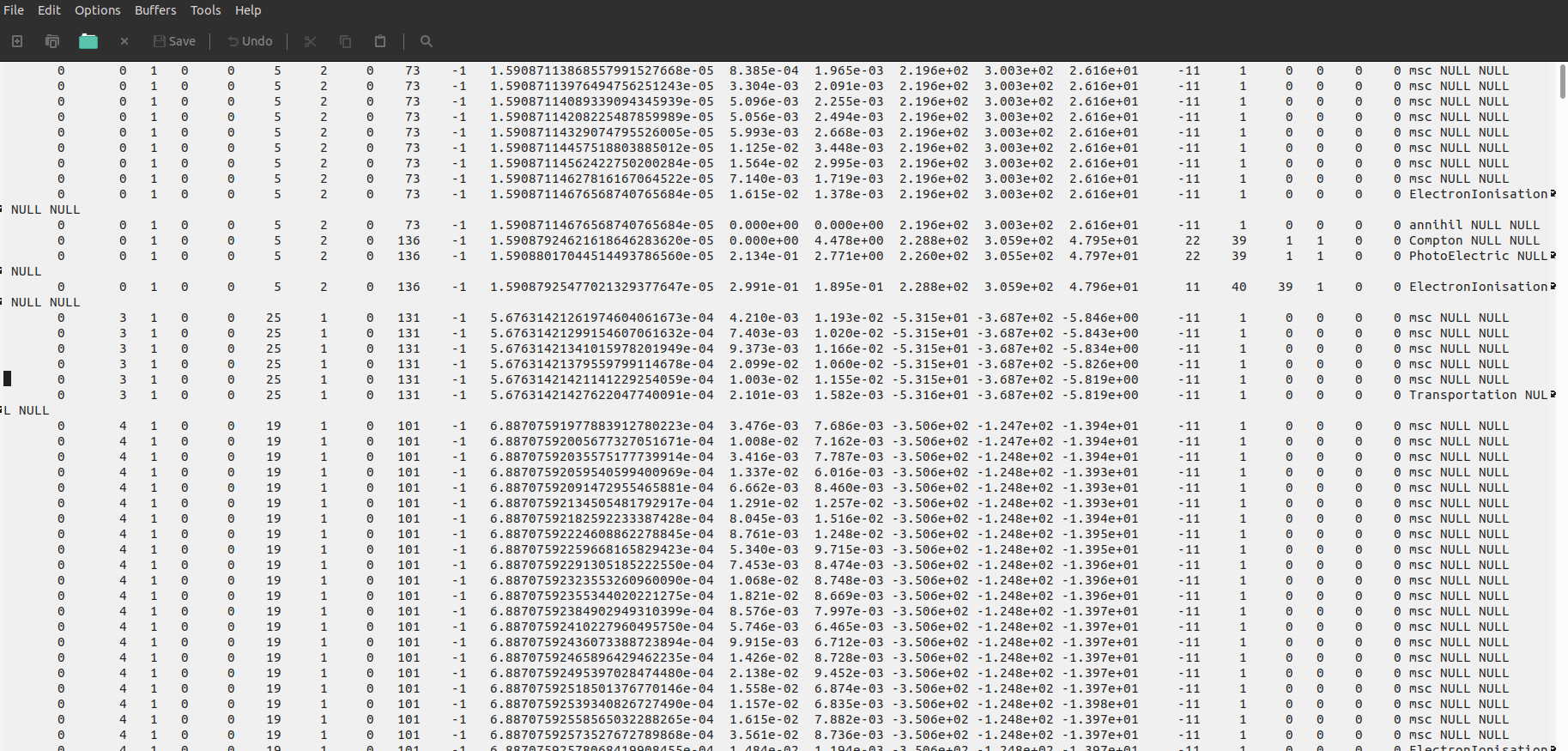
上の図はOUTPUTNAMEHits.datを開いた結果を示します。数字の羅列です。各列が何を示しているのかはサンプルコードの種類（PETやSPECTなど）で変わってきます。こちらに一覧が載っています。
The figure above shows the result of opening OUTPUTNAMEHits.dat. It is a list of numbers. What each column shows depends on the type of sample code (PET, SPECT, etc.). You can see the list here.
-> 4.1.1. Description of the ASCII(binary) file content

1列目 : ID of the run (i.e. time-slice)
2列目 : ID of the event
3列目 : ID of the primary particle whose descendant generated this hit
4列目 : ID of the source which emitted the primary particle
5～N+4列目 : Volume IDs at each level of the hierarchy of a system, so the number of columns depends on the system used.

などなど、続きます。
データ容量が多いのでASCII形式は非推奨です。
The size of ASCII data is too big, so I don’t recommend it.

以下のようにsetOutFileSingles[digitizer_module_name] 1とすると
If you write “setOutFileSingles[digitizer_module_name] 1” in your macro file …

/gate/output/ascii/enable
/gate/output/ascii/setFileName  OUTPUTNAME
/gate/output/ascii/setOutFileSinglesAdderFlag 1
/gate/output/ascii/setOutFileSinglesBlurringFlag 1
/gate/output/ascii/setOutFileSinglesThresholderFlag 1
/gate/output/ascii/setOutFileSinglesUpholderFlag 1

先ほどのファイル（OUTPUTNAMEXXXXX.dat）以外に以下のもの（OUTPUTNAMESinglesXXXXX.dat）が出力されます。これらはDigitizerモジュールを通過した後の値であり、デバッグに有用です。
In addition to the above result (OUTPUTNAMEXXXXX.dat), the following (OUTPUTNAMESinglesXXXXX.dat) is output. These are the values after passing through the Digitizer module and are useful for debugging.
・OUTPUTNAMESinglesAdder.dat
・OUTPUTNAMESinglesBlurring.dat
・OUTPUTNAMESinglesThresholder.dat
・OUTPUTNAMESinglesUpholder.dat
全部を保存しようとすると、その分データ容量は大きくなりますので注意です。
If you try to save all the data, the size of the data will be very large. Please be careful.

ROOT形式（推奨）
　　（recommend）

ROOT形式は全てのサンプルコードで出力可能です。扱いには少し練習が必要ですが、ASCIIファイルよりも容量が小さく、様々な角度(条件)から図を作成することができます。
ROOT format can be output with all sample code. It takes a little practice to handle, but it is smaller than an ASCII file and you can create diagrams from various conditions.

/gate/output/root/enable
/gate/output/root/setFileName  OUTPUTNAME
/gate/output/root/setRootHitFlag            1
/gate/output/root/setRootSinglesFlag        1
/gate/output/root/setRootCoincidencesFlag   1
/gate/output/root/setRootNtupleFlag         1

# for debug
/gate/output/root/setOutFileSinglesAdderFlag         0
/gate/output/root/setOutFileSinglesReadoutFlag       0
/gate/output/root/setOutFileSinglesSpblurringFlag    0
/gate/output/root/setOutFileSinglesBlurringFlag      0
/gate/output/root/setOutFileSinglesThresholderFlag   0
/gate/output/root/setOutFileSinglesUpholderFlag      0

それぞれ出力したい情報（Hits、Singles、Coincidences、Ntuple）のFlagを1とするとデータが蓄積されます。全部を保存しようとすると、その分データ容量は大きくなりますので注意です。
出力されるのは１つのROOTファイルです。
この場合は「OUTPUTNAME.root」という名前になります。
If you set the Flag of the information you want to output (Hits, Singles, Coincidences, Ntuple) to 1, the data will be accumulated. Note that if you try to save all, the data capacity will increase accordingly.
Only one ROOT file is output.
In this case, it will be named “OUTPUTNAME.root”.

Hits,Singles,Coincidencesでそれぞれ格納している情報が違います
The information stored in Hits, Singles, and Coincidences is different.

補足として
PDGEncoding: 粒子の種類　types of particle ex) gamma=22, electron=11
edep: energy deposit (エネルギー付与）
localPosX: 娘Volumeの内部のX座標
　　　　　　　　　　　　　　<—> posX or globalPosX: WorldのX座標
processName: 相互作用の名称 names of process

ROOTファイルの操作
　　　Handling ROOT files

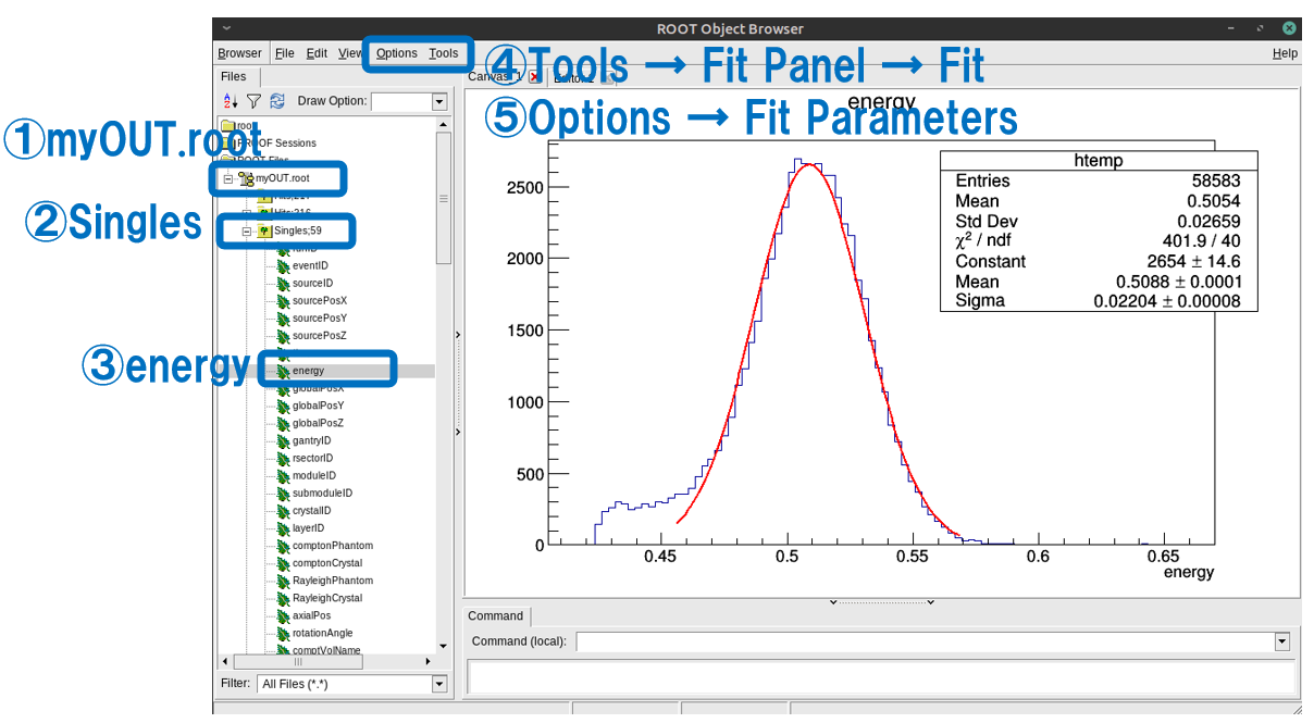
この自作CylinderPETから得られたmyOUT.rootを開いてみましょう。
Let’s open myOUT.root obtained from this edited Cylinder PET.

myPET_DMI.mac ダウンロード

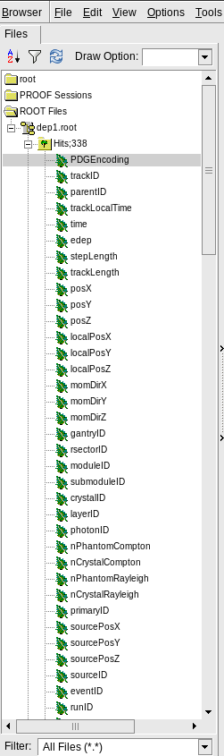
root myOUT.root

ROOTファイルの中身をざっと確認するにはGUIを使う方法がおすすめです。
It is recommended to use the GUI to roughly check the contents of the ROOT file.

TBrowser tb;

「tb」というのは名前のようなものなので、なんでもOKです。
TBrowser hogehoge; でもOK
“Tb” is like a name, so you can name it freely.
ex) TBrowser hogehoge;

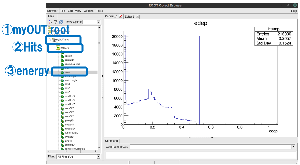
Hitsのenergyを表示してみました。まだ、digitizerを通ってないのでエネルギーピークは鋭いですね。
I showed Hits energy. The energy peak is sharp because it has not passed through the digitizer yet.

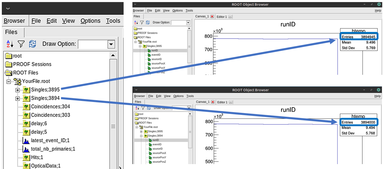
ちなみにそれぞれの項目に関して２つ項目（leaf）ができているのは切りのいい数値で保存しているからのようです。「Singles」の後ろの数値(3894)に1000を掛けたものがデータ数を表しています。
By the way, it seems that two items (leaf) are made for each item because they are saved with nice round number. The number after the “Singles” (3894) multiplied by 1000 represents the number of data.

SinglesはDigitizerの処理にエネルギー分解能を含めているためスペクトルに広がりがでています。また、Threshold=0.42MeVかつUphold=0.65MeVとしていますので、その範囲しかデータがありません。
The energy of “Singles” is blurred by the processing of “Digitizer”. Also, there is only data in the range between Threshold and Uphold.

このような感じでGUIで簡単に結果を確認することができます。
As shown above, we can see the results easily by GUI.

しかし、もっと詳細にデータを表示するためにCUIを使います。
However, you can analyze it in more detail by using CUI.

.ls

TFile**		myOUT.root	ROOT file with histograms
 TFile*		myOUT.root	ROOT file with histograms
  OBJ: TTree	Hits	The root tree for hits : 0 at: 0x5618feb938a0
  OBJ: TTree	Hits	The root tree for hits : 0 at: 0x5618fe6cd750
  OBJ: TTree	Singles	The root tree for singles : 0 at: 0x5618fd4a9d90
  OBJ: TTree	Singles	The root tree for singles : 0 at: 0x5618fe50d3c0
  KEY: TTree	Hits;217	The root tree for hits
  KEY: TTree	Hits;216	The root tree for hits
  KEY: TTree	Singles;59	The root tree for singles
  KEY: TTree	Singles;58	The root tree for singles
  KEY: TTree	Coincidences;5	The root tree for coincidences
  KEY: TTree	Coincidences;4	The root tree for coincidences
  KEY: TH1D	latest_event_ID;1	latest_event_ID(#)
  KEY: TH1D	total_nb_primaries;1	total_nb_primaries(#)
  KEY: TTree	OpticalData;1	OpticalData
  KEY: TTree	delay;1	The root tree for coincidences

どのような構造になっているか確認するためには「.ls」と打ちます。ピリオドを忘れないでください。
You can use the “.ls” command to check the structure of the output data. Please do not forget to put the ” . ”

この結果からTTree（枝や葉っぱを持つ木のような）としてHits, Singles, Coincidences, delay, Hitsなどがあることが分かります。
これらのTTreeはさらにいろいろな情報を持っています。
As you can see from this result, you can see that Hits, Singles, Coincidences, delay, Hits, etc. are stored in the form of TTree (like a tree with branches and leaves).
These TTrees also have various branches.

どんなデータを持っているかを表示するにはPrint()関数を使用します。使い方は以下の通りです。（先ほどのTBrowserで確認しておくのも良い）
Use the “Print” function to display what data each “TTree” has. The usage is as follows. (It is ok to check it with TBrowser in advance.)

Hits->Print();

すると、以下のように表示されます。
then, you see the results as bellow.

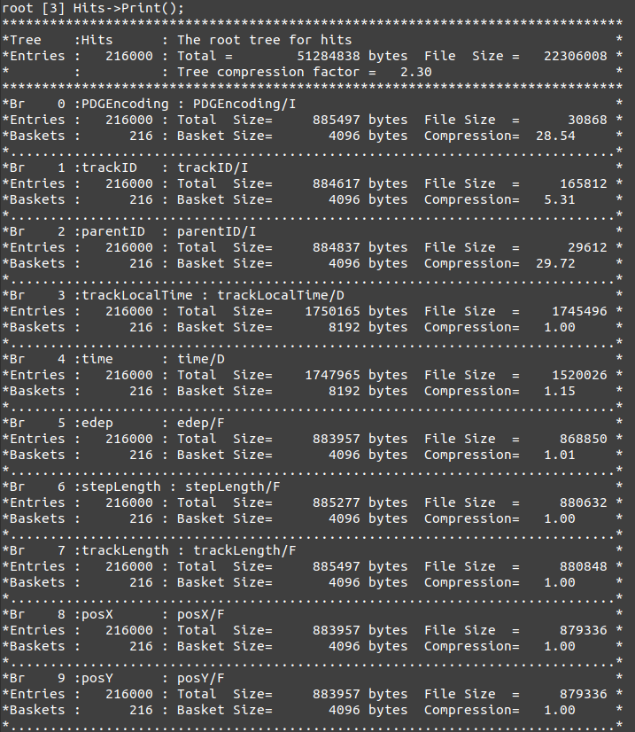
長すぎて、全部表示できていませんが、どのような枝（Br：Branch）があるのが分かります。
There are too many lines to display them all, but you can see what kind of branch (Br: Branch) there is.

次に図を描いていきます。
Next, you draw the figure by “Draw” command.

Hits->Draw("posX")

そうすると
then

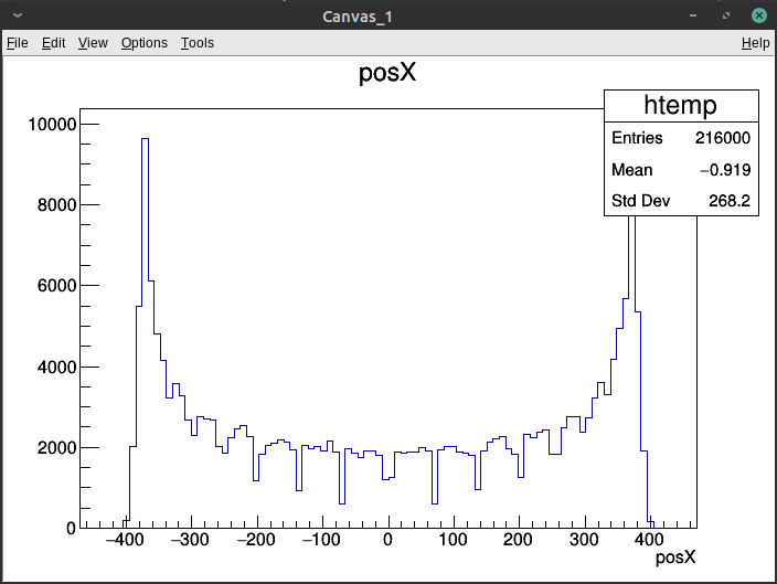
Hitsが起こったX座標が出力されました。縦軸は頻度です。
The location (X coordinate) where the Hit information was generated is output. The vertical axis is frequency.

次に軸を増やします。
You can display in two dimensions as follow.

Hits->Draw("posX:posY");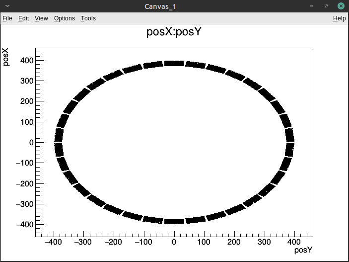

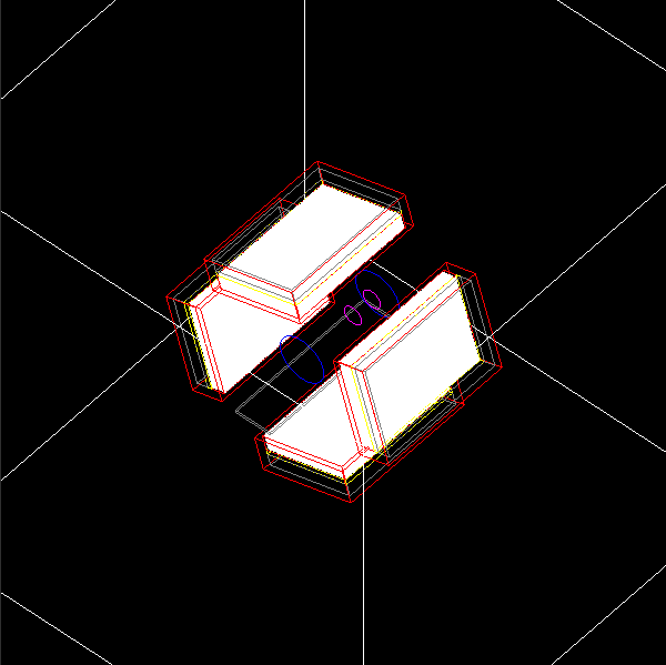
次は三次元です。
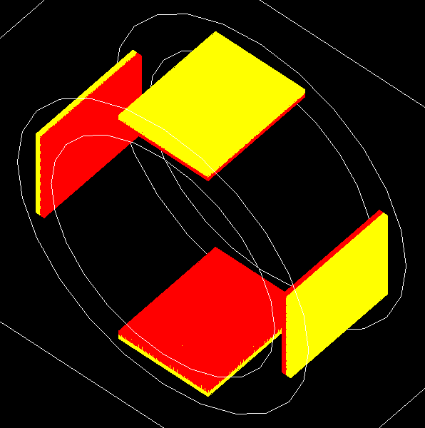
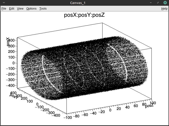
Next, 3D images.

Hits->Draw("posX:posY:posZ");

このように「:」で繋げると、3次元まで増やすことができます。
In this way, if you connect sentence with “:”, you can increase dimensions up to three.

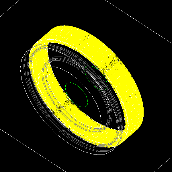
さらに2番目の引数を与えることで、表示条件を変更することができます。
You can change the display condition by giving the second argument.

Hits->Draw("posX:posY:posZ","time<1");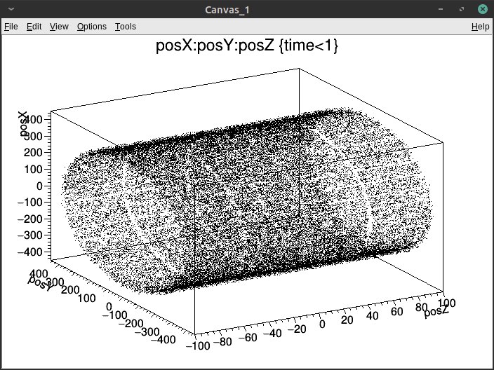

撮像時間（time）を1秒未満という条件を加えました。カウントが少なくなって、色が薄くなりましたね。
The count has decreased and the color has become lighter by adding the limitation “time (imaging time) <1”

さらにファントムの中で、散乱したという条件を加えると。
If you add the limitation that the Compton scattering is occurred inside the phantom.

Hits->Draw("posX:posY:posZ","time<1&&0<nPhantomCompton");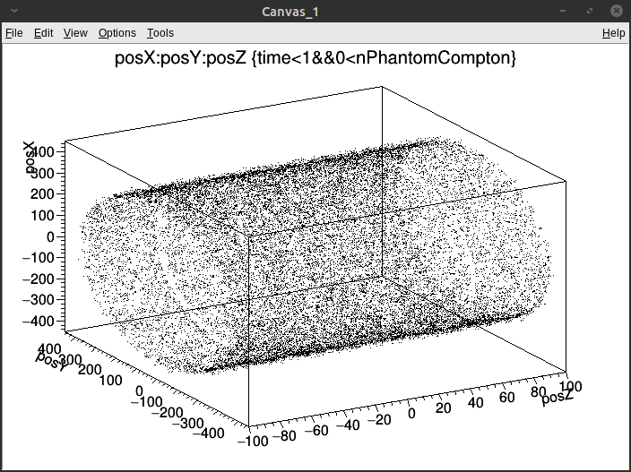

このように他の枝の値を使って条件をいくつでも追加していくことができます。
As shown, adding the branch as limitation, you can change the condition to display figure.

3つ目の引数を与えると図の表示法を変えることができます。
You can change the way to display figure by giving a third argument.

ここに示した以外の方法もたくさんありますのでROOTの公式ページを見てください。
There are many methods other than those shown here, so please see the official ROOT page.

Hits->Draw("posZ","time<1","")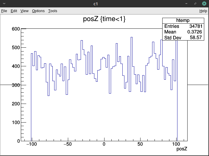

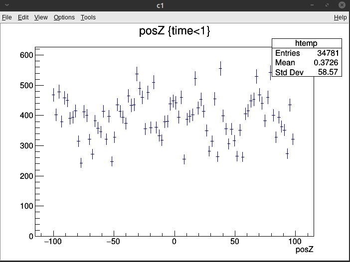
Hits->Draw("posZ","time<1","e")

「e」でエラーバーが付きます
The argument “e” adds an error bar to the figure.

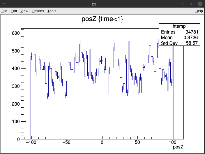
 Hits->Draw("posZ","time<1","histe")

「hist+e」でエラーバー付きのヒストグラムとなります。
Histogram with error bars when using “hist + e”.

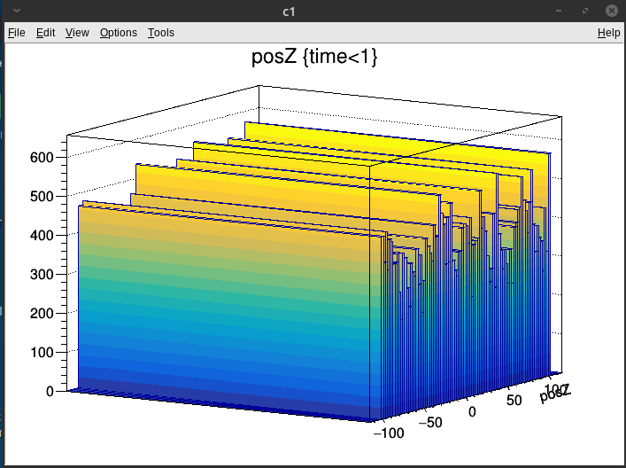
Hits->Draw("posZ","time<1","lego")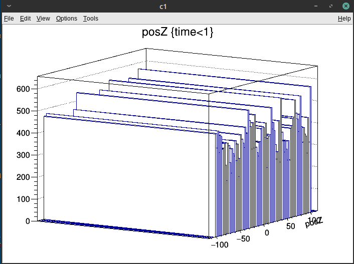

Hits->Draw("posZ","time<1","lego2")

lego3もあります
You can also use “lego3”.

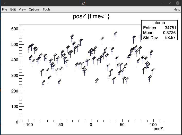
Hits->Draw("posZ","time<1","text45")

45は角度を表しています（0 < angle < 99）
“45” means the text angle. (0 < angle < 99)

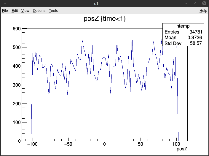
Hits->Draw("posZ","time<1","l")

Lineです。
“l” means line.

Hits->Draw("posX:posY","time<1","box")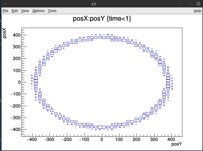

 Hits->Draw("posX:posY","time<1","colz")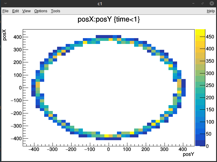

Hits->Draw("posX:posY","time<1","lego2")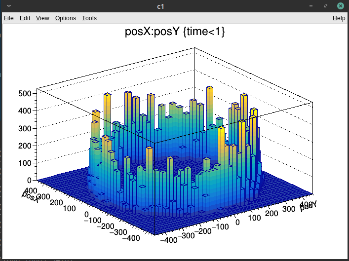

Hits->Draw("posX:posY","time<1","cont1")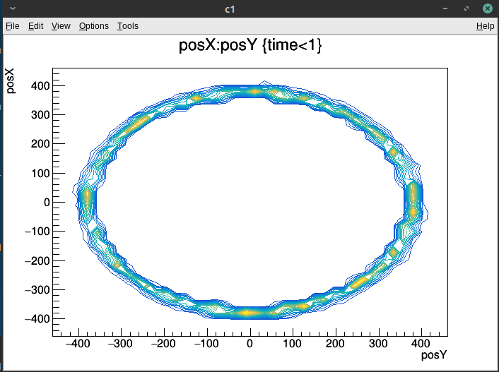

Hits->Draw("posX:posY","time<1","surf3")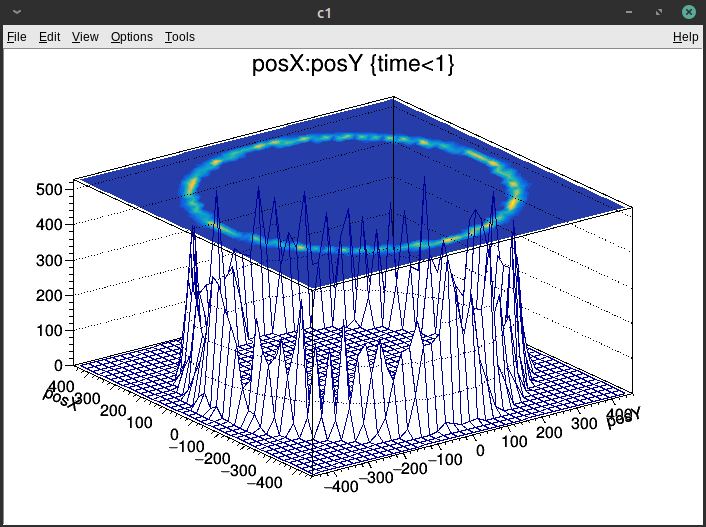

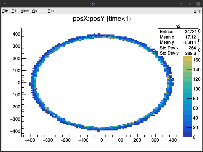
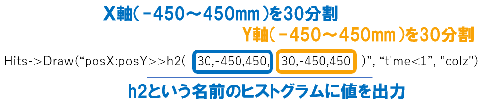
ヒストグラムのbinを指定して図を作成します。
上が-450mm~450mmの範囲を30個に分けた場合、
下が100個に分けた場合です。
Create a diagram by specifying the bin of the histogram.
The figure above shows the range from -450mm to 450mm divided into 30 pieces.
The case below is divided into 100 pieces.

Hits->Draw("posX:posY>>h2(30,-450,450,30,-450,450)","time<1","colz")
Hits->Draw("posX:posY>>h3(100,-450,450,100,-450,450)","time<1","colz")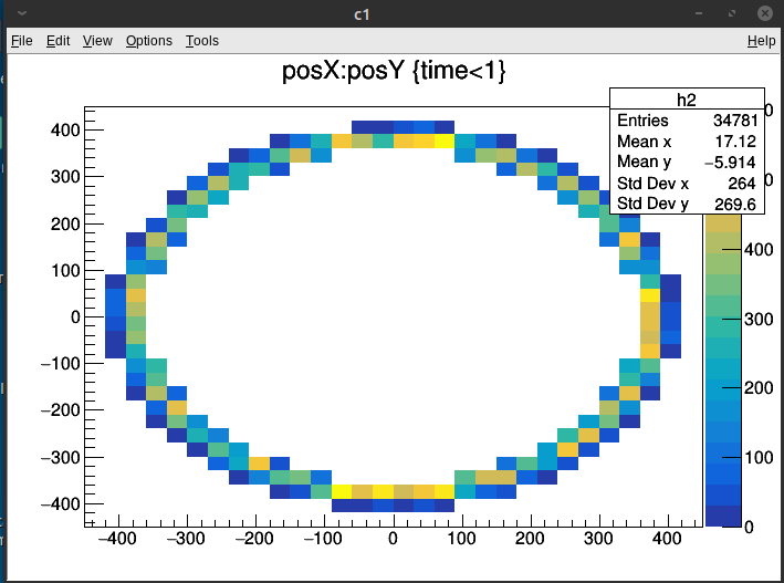

sinogramThetaとsinogramSの順番を変えると・・・
If you change the order of “sinogramTheta” and “sinogramS”…

Coincidences->Draw("sinogramS:sinogramTheta>>h5(20,0,3,100,-300,300)")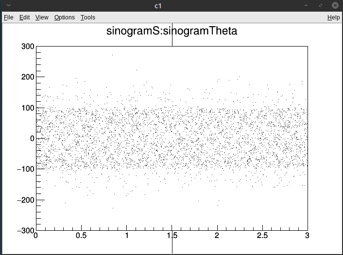

h5というTH2インスタンスに情報が格納されているので・・・
The data is contained in a TH2 instance named “h5”.

h5->Draw("candlex(2001)");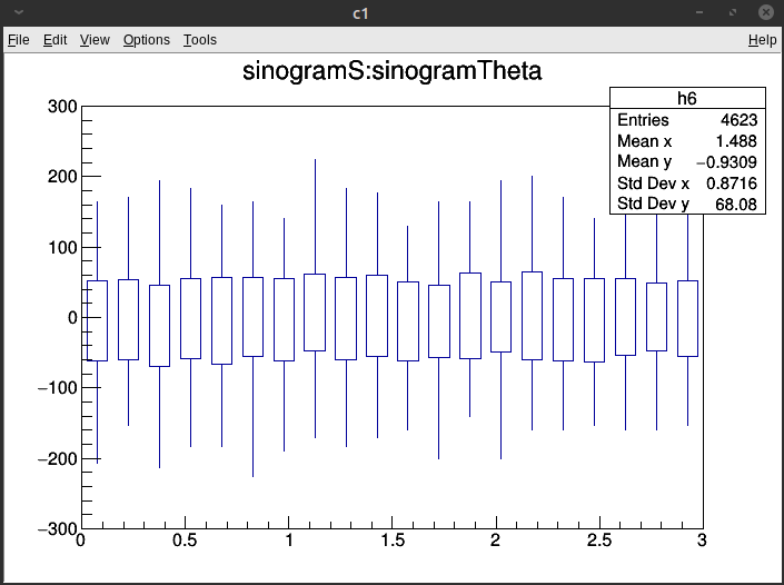

箱ひげができました。
Box plot is made.

最後にヒストグラムをテキストファイルに出力する方法を示します。
Finally, I shows how to output a histogram to a text file.

vgate:~/GateContrib/imaging/myPET > root myOUT.root

として、ROOTファイルを開いたあと
after you open the root file…

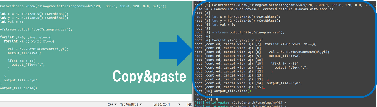
マクロファイルに記述して読み込ませるのが普通だと思いますが、上手くいかなかったので以下のコマンドを一度に全部コピペしてください。
必要に応じて、分割数や範囲、出力ファイル名を変更してください。
I think that it is the usual way to write it in a macro file and read it, but since it did not work well, please copy and paste the following commands all at once.
Change the number of divisions, the range, and the output file name as necessary.

histout ダウンロード


Coincidences->Draw("sinogramTheta:sinogramS>>h2(128, -300.0, 300.0, 128, 0.0, 3.1)");

int x = h2->GetXaxis()->GetNbins();  
int y = h2->GetYaxis()->GetNbins();  
int val = 0;

ofstream output_file("sinogram.csv");

for(int yi=0; yi<y; yi++){
  for(int xi=0; xi<x; xi++){

    val = h2->GetBinContent(xi,yi);
    output_file<<val;

    if(xi! = x-1){
      output_file<<",";
    }

  }
  output_file<<"\n";
}
output_file.close()

上の例ではsinogram.csvという名前で保存されているので、ImageJで開きましょう。
In the above example, it is saved as a file named sinogram.csv, so let’s open it with ImageJ.

vgate:~/GateContrib/imaging/myPET > imagej

imagejと打ちます。
（vGATE9.0ではImageJ(Fiji)がすでにインストールされています。）
Please put “imagej”．
（ ImageJ(Fiji) is already installed in vGATE9.0 ）

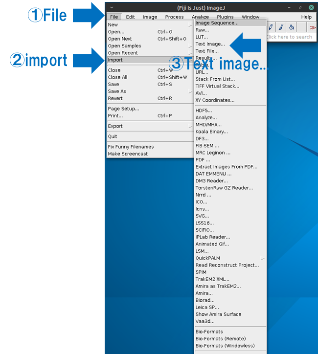
File->import->Text image…の順に進み、sinogram.csvを開いてください。
You open sinogram.csv by “File->import->Text image…”.

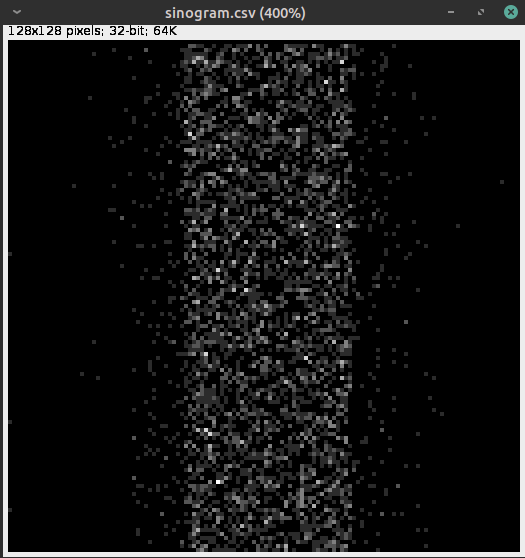
確認できました。
Successful.

Interfile形式

SPECTheadで出力できます。
You can specify the interfile format as output in SPECThead.

以下のコマンドがInterfileの出力コマンドに該当します。
The following command outputs Interfile.

# P R O J E C T I O N
#####
/gate/output/projection/enable
/gate/output/projection/setFileName 　OUTPUTNAME
/gate/output/projection/pixelSizeX 0.904 mm
/gate/output/projection/pixelSizeY 0.904 mm
/gate/output/projection/pixelNumberX 128
/gate/output/projection/pixelNumberY 128

# Specify the projection plane (XY, YZ or ZX)
##
/gate/output/projection/projectionPlane YZ

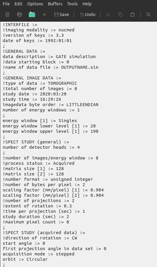
上の例ではOUTPUTNAME.hdrとOUTPUTNAME.sinが出力されます。
.hdrはヘッダーファイルでASCII形式なのでテキストエディタで中身を確認することができます。
In the above example, OUTPUTNAME.hdr and OUTPUTNAME.sin will be output.
Since .hdr is a header file in ASCII format, you can check the contents with a text editor.

gedit  OUTPUTNAME.hdr

と打って
then

rawデータ自体は「.sin」の方に保存されています。このデータを開くためには「.hdr」ファイルの情報が必要です。Intefileを開く方法の1つはImageJを使用することです。このページも見てください。
Raw data itself is stored in “.sin”. The information in the “.hdr” file is required to open this data. One way to open an Intefile is to use ImageJ. See also this page.

imagej

としてImageJ(Fiji)を起動します
You run the ImageJ(Fiji).

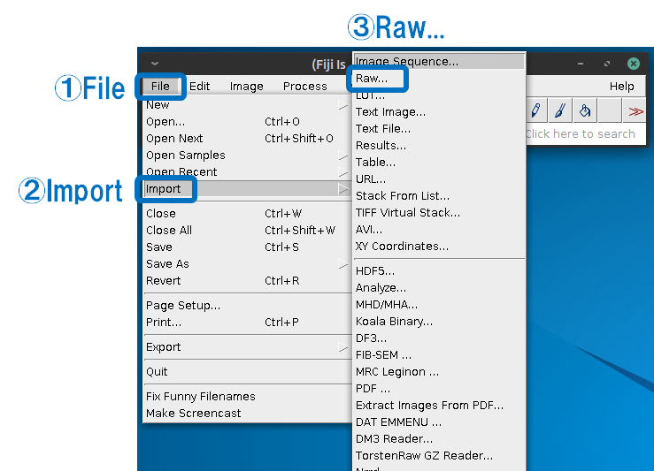
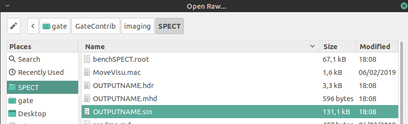
OUTPUTNAME.sinを選択します。ヘッダーファイルではなく。
Select OUTPUTNAME.sin instead of the header file.

先ほどのOUTPUTNAME.hdrの内容を見ながら以下のように入力します。
Enter the following while looking at the contents of OUTPUTNAME.hdr .

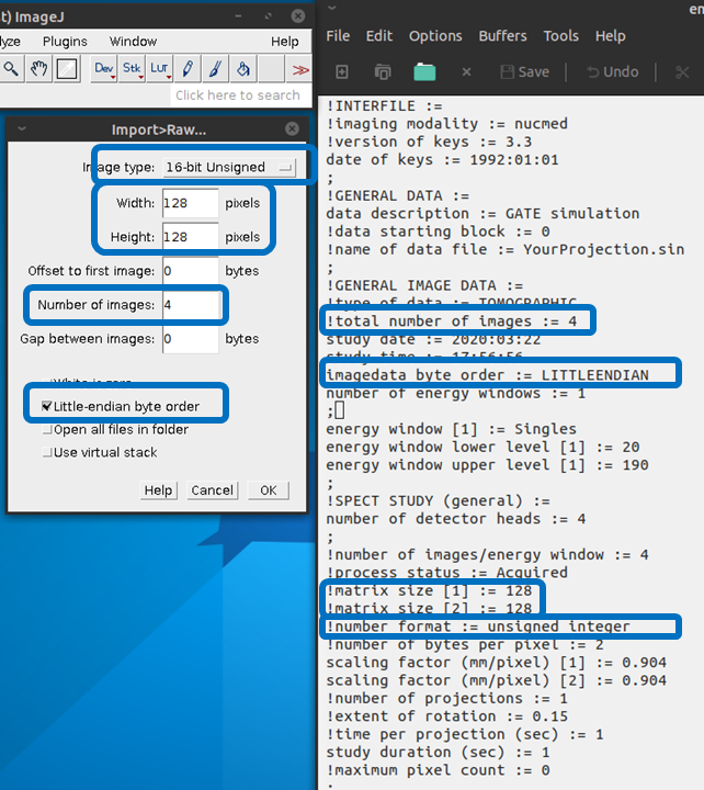
これで画像が開かれます。
Image will be opened.

admin_bear

この他にも
・Sinogram形式
・Ecat7形式
・LMF形式
などありますが、使ったことないのでまだ今度
There are above format, but I have not used it yet

numpy形式

pythonで扱うことができる形式です。
以下の文をOUTPUTに記載すると「p.hits.npy」と「p.Singles.npy」が出力されます
It is a format that can be handled by python.
When the following sentence is described in OUTPUT, “p.hits.npy” and “p.Singles.npy” are output.

#####OUT PUT#################
/gate/output/tree/enable
/gate/output/tree/addFileName   p.npy
/gate/output/tree/hits/enable
/gate/output/tree/addCollection Singles

ファイルを開くにはpythonを使いますが、どうやらnumpyがインストールされていないようです。そのためにはpipが必要で・・・・
とにかく以下のコマンドを打ってください。
I need numpy to open the file, but numpy is not installed. Pip is required for installation.
Type the following command.

sudo apt install python-pip

pip install numpy

numpyがインストールされたらpythonを起動します
Start python after installing numpy.

python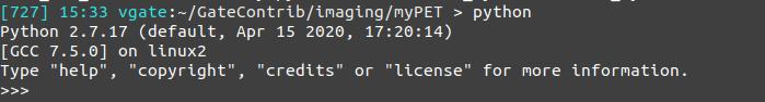

>>>　と表示されたら
When ” >>> ” is shown

import numpy

と打ってnumpyをインポートします。
You import numpy.

hits = numpy.load("p.hits.npy")

で「p.hits.npy」をhitsに格納します。
どんなデータが入っているのかを確認すると
Store “p.hits.npy” in the “hits” variable.
If you check what kind of data it contains

>>> numpy.info(hits)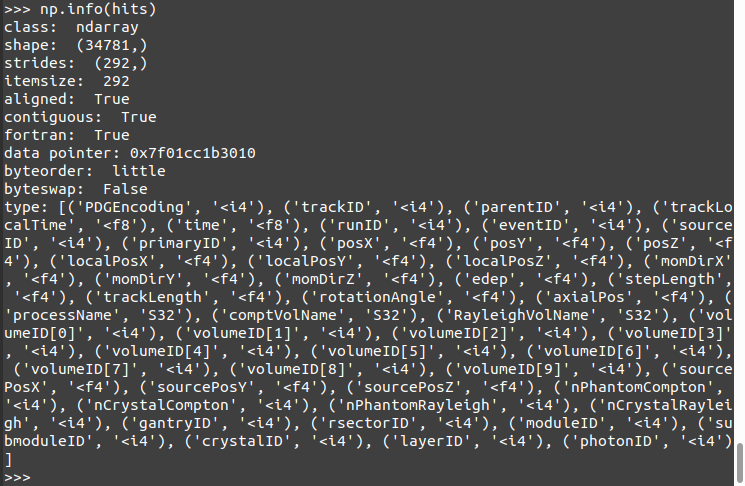

こんな情報が含まれています。
このデータを使ってどういう解析をするのかは、また勉強して書きたいと思います。
The above information is contained in the hits variable.
I would like to study and write again what kind of analysis is to be done using this data.

admin_bear

では、今日はこれまでにします。
Bye for now !

GATEの使い方 5 ~結果の出力と表示~

出力形式の指定
　　　Specify the output format

ASCII形式（推奨しない）
　　(not recommended)

ROOT形式（推奨）
　　（recommend）

ROOTファイルの操作
　　　Handling ROOT files

Interfile形式

numpy形式

SIMINDの使い方１～ダウンロードとインストール～

ImageJの使い方 2　ーEditメニュー編ー

画像再構成ソフトウェア～TIGRE～

COMMENT コメントをキャンセル

あなたは医療従事者ですか？

出力形式の指定 Specify the output format

ASCII形式（推奨しない） (not recommended)

ROOT形式（推奨） （recommend）

ROOTファイルの操作 Handling ROOT files

Interfile形式

numpy形式

SIMINDの使い方１ ～ダウンロードとインストール～

ImageJの使い方 2 ーEditメニュー編ー

画像再構成ソフトウェア ～TIGRE～

COMMENT コメントをキャンセル

Radiography

GATEの使い方 １ ~vGATEの環境構築~

【雑記】診療放射線技師としての働き方 ～高校生から社会人3年目の方へ～

撮影法

【検証】一般撮影におけるX線中心の推定

出力形式の指定
　　　Specify the output format

ASCII形式（推奨しない）
　　(not recommended)

ROOT形式（推奨）
　　（recommend）

ROOTファイルの操作
　　　Handling ROOT files

SIMINDの使い方１～ダウンロードとインストール～

ImageJの使い方 2　ーEditメニュー編ー

画像再構成ソフトウェア～TIGRE～

GATEの使い方１ ~vGATEの環境構築~

【雑記】診療放射線技師としての働き方　～高校生から社会人3年目の方へ～